The basic ideology behind Natural Language Processing (NLP) is to teach machines to understand human language in written or spoken form and to derive meaning from it.

So the inputs and most of the features in NLP tasks are textual, be it words, n-grams, letters or Part of Speech (POS) tags etc. But machines can only understand numbers and not alphabets or words. Machine learning models take real valued vectors as input. So we need to translate our language to theirs, for them to make sense out of it. We need a process which maps the textual data to real valued vectors. This process is what we call word representation or feature extraction in NLP based problems.

This post provides an overview of the different possible approaches to word representation in NLP. The approaches have been loosely classified into the following categories:

1. Count-based methods - Sparse encodings

   • Bag of words

2. Distributional semantics methods

   • Co-occurrence matrix
   • Pointwise Mutual Information (PMI)
   • Term Frequency - Inverse Document Frequency (TF-IDF)

3. Dense encodings - Dense word embeddings

   • Singular Value Decomposition (SVD)
   • Word2Vec
   • GloVe

Note that different resources might provide different categorizations, but I find this the most suitable. Regardless, I have tried to cover all the popular methods in a comprehensive manner here.
This article is the first in a series of two articles:

1. THIS - Discusses sparse encodings and distributional semantics methods.

2. Part 2 - It will be coming soon, with discussion about dense encodings techniques.

Basic Concepts

Let us first see some basic terms that will be used in the rest of the article.

1. Corpus - In simple language, corpus is a large collection of texts that has been accumulated from various written, spoken or other natural language sources and assembled in a structured manner.

2. Document - Each instance in the corpus is a document. A document can contain any number of sentences.

3. Context - A context is the neighbourhood in a specified window size, that is to be taken into consideration while finding representation of a word. For eg. for a word, words on its either side could be its context. For a sentence on the other hand, we might call its surrounding sentences as context.

. . .

Count-based methods (Sparse encodings)

Sparse encodings are the simplest approaches to word representation. They are very high dimensional representations.

Bag of words

Here we first form a bag of all unique words that we extract from all the documents in the corpus. Let us take different reviews of a travel destination as our example:

Document 1: Munnar is the most mesmerizing hill station.
Document 2: Munnar National park is a waste of time.
Document 3: Magnificent view of the peaks in Munnar.

The bag of words vector will be of size 1XN, where N=Size of vocabulary.
Let’s do a very basic pre-processing to begin with, by converting all the words to lowercase and then build a bag of words from the above documents:

• munnar
• is
• the
• most
• mesmerizing
• hill
• station
• national
• park
• a
• waste
• of
• time
• magnificent
• view
• peaks

We can see the vector size is 1X16. Now a simple way to represent each of the words is to construct a vector the size of the vocabulary, where only the digit at the same index as the index of the word in the vocabulary will be 1 and the rest of the digits will be 0.

Word	One-hot vector
munnar	[1, 0, 0, 0, 0, 0, 0, 0, 0, 0, 0, 0, 0, 0, 0, 0]
hill	[0, 0, 0, 0, 0, 1, 0, 0, 0, 0, 0, 0, 0, 0, 0, 0]
time	[0, 0, 0, 0, 0, 0, 0, 0, 0, 0, 0, 0, 1, 0, 0, 0]
peaks	[0, 0, 0, 0, 0, 0, 0, 0, 0, 0, 0, 0, 0, 0, 0, 1]

We have formed a binary vector, giving the One-hot encoding, indicating whether a word is present in a sentence or not. But there can be various other methods to convert the bag of words into a word representation. We can have a frequency distribution vector, called Count vector, indicating how many times the word appeared in that document rather than just indicating the presence or absence of the word. Another technique is TF-IDF, which we will discuss in detail at a later stage in this article.

This is the most basic feature extraction technique. Problems with this technique?

• What happens when the vocabulary size is substantially large, maybe millions of words? Apart from the obvious storage problem, this representation might also trigger the phenomenon of the curse of dimensionality.
• Now the vector will likely be a sparse matrix, and it is computationally hard to model sparse data in deep learning and it is hard to generalize with sparse input.
• Can you think of any other problem with such a representation? What happens if another word gets added to the vocabulary? And another? Yeah, it’s not a scalable representation.
• Now let’s try to understand a bigger problem. This representation is a vector. In vectors, we can talk about similarity between 2 vectors. The similarity measure could be cosine similarity, euclidean distance or any other similar method. Let’s consider cosine similarity between the vector representation of peaks, hill and time. All the cosine similarities come out to be 0, as all the one-hot vectors are orthogonal. But ideally, wouldn’t we want the vector for peaks to be a little more similar to hill than to time, given they are similar in meanings?

So the count vector model is giving us no information about the meanings of words and we are essentially losing a large amount of data just like that. We surely need a better representation that numerifies syntactic and semantic information as well.

Distributional semantic methods

This is an umbrella word for any type of technique that models the meaning of the word in its vector representation. Let us see where its intuition is coming from.
You are given two sentences:

Sentence 1: The team discussed their immediate goals for next month.
Sentence 2: The company missed the annual target this appraisal season.

From these sentences, we can see that since the words target and goal are being used in a similar environment, they might have similar meanings too.

“You shall know a word by the company it keeps.”

Firth, J.R., 1957:11

Co-occurrence Matrix

In Linear algebra, co-occurrence matrix is a matrix that is used to store how many times a particular pair of entities did an event together.
Example:
Let’s assume we have a column dedicated to each actor in the Bollywood industry, and a row dedicated to each of the actresses and we store the number of movies actress i has ever done opposite actor j. Therefore,

Entities = Actors and actresses,      Event = Movie

What we get after populating all the elements is a co-occurrence matrix, telling us about pairings in Bollywood movies.
Similarly, we use a co-occurrence matrix in NLP, to store how many times a pair of words occurs together in a document. In this case,

Entities = Words,      Event = Occurrence in common documents

Consider the previous example regarding reviews of a travel destination. If we consider the context of the word national, we can see the words munnar, park, is, a, waste, of and time. So in the co-occurrence matrix, for the word national, we will see the entries corresponding to these words in its context to be 1 and the rest will be 0.

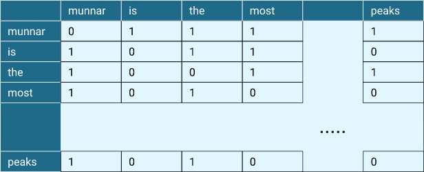
Figure 1: Co-occurrence matrix showing representation for some of the words from our example

But in reality, do all the words in a document contribute to the meaning or context of a word? Probably not. We can infer the meaning of a word by looking at a small context occurring around it.
Hence we also define the concept of a Context Window, which tells how many neighbours of a word we are taking into consideration. So now we are looking at how many times a pair of words appears together in a context window.

To understand it better through our example, let us take window size = 2. This means, we are now considering two words to the left and two to the right for our current word. So the context words for national can be written as:

Word	Context
national	munnar(1), park(1), is(1)

This type of a co-occurrence matrix is called Term-Context matrix, where we have defined the context. The previous one is called Term-Document matrix, because in that case the whole document is the context for the word. Now we have obtained a co-occurrence matrix of size NXN, where N=Size of vocabulary.

Let us see the drawbacks of this model.

• Co-occurrence matrix is less sparse than one-hot encoding but it is still sparse, because not all words will appear in a word’s context. Hence many of the entries will be 0.
• Other than that, there are words like i, is, are, to in the context matrix, which we call stop words and which do not really have any contribution to the meaning or sentiment of words, or the document in general. But they appear very frequently in any corpus, so their count in the matrix will be very high. You can already see how that’s a problem. Say you wanted to get an idea of the contexts that are shared by the words wayanad and munnar. But the stop words occur frequently with all sorts of words and also in the context of these two words. So they would skew the raw frequency values we stored in the co-occurrence matrix.
• Similarly, you wanted to know if the word united occurring together with states frequently is showing some sort of unique pattern or is it just as meaningless as some states or these states. How would you be able to assess such a pattern with raw frequencies? You might want a better parameter than raw frequencies, which tells you whether two words co-occur by chance, or they provide a unique concept.

We can deal with these problems in one of the following ways:

1. We might ignore very frequent words in the co-occurrence matrix.
2. We may use thresholding to say that if any word in the context has a frequency higher than let’s say t, we will take it as t rather than the actual word count. So we are no more interested in keeping the count of that word.
3. We might form an exhaustive list of stop words and remove those from our corpus before we form the vector representation.
4. We can also solve this problem using different methods which are used to assign importance to words. We can use PMI and TF-IDF, which we will be discussing in the next sections.

Apart from the above mentioned problems and their solutions, co-occurrence matrix also suffers from all the problems that were presented in the one-hot encoding method - scalability issues, high dimensional representation and sparsity. To solve these, we might want to apply decomposition techniques such as SVD (Singular Value Decomposition) and reduce the dimensionality of the co-occurrence matrix. We will have a look at SVD in a later section.

Pointwise Mutual Information (PMI)

In general, PMI is the measure of correlation between two events. It tries to quantify whether two events occur more in each other’s presence, than when they are independent. In our case, the event would be the occurrence of two words together in each other’s context. So PMI between two words tries to find out how often two words co-occur.
Equation 1: Equation 2:
Equation 1 is the original form of the mathematical formula for PMI. It can also be written in the form presented in equation 2.

To understand the concept and its necessity in a better way, let us go back to the example we saw in the co-occurrence matrix. Let us consider the bigram expression united states. We want to understand whether the occurrence of both the words in this expression is depicting a special pattern. Yes, both the words united and states have individual meaning and existence, but when they occur together, do they represent a unique meaning? If they are, is the expression many states also a unique occurrence and an important concept? If not, how exactly do we quantitatively differentiate between both?
Another example - we see in a corpus that the expression new zealand occurs frequently. Why is that? Is it only because new is a frequent word and thus has a higher chance to occur with other less important words, just like many states in the previous example? Or is new zealand actually a unique concept worth its own existence irrespective of the frequency of both the constituent words?
This is what PMI is trying to solve. We already saw that PMI is trying to capture the likelihood of co-occurrence of two words. The formula might give a better intuition as to what PMI captures.

The range of PMI is [-∞, ∞]. Let us now see different possible cases to get a better grip of how PMI varies with various word frequencies.

1. If two words appear a lot individually, but not much together, their individual probabilities P(word1) and P(word2) will be high. Their joint probability P(word1, word2) however will be low in this case. Hence the PMI is going to be negative.
2. If both the words occur less frequently, but both occur together at a high frequency, they are probably representing a unique concept. Looking at the formula, P(word1) and P(word2) will be low, but P(word1, word2) will be high, resulting in a high positive PMI score.
3. If one of the words has a very high frequency, resulting in a higher co-occurrence of both of the words, we will have a high P(word1), a low P(word2) and a high P(word1, word2). So the overall PMI score will be low. This also means that the stop words and their likes will now have a low PMI in the context of a word.
4. If two words occur independent of each other, we know that their joint probability can be given by the following formula
   Equation 3: So the ratio inside the log will be 1, resulting in a 0 PMI score.
5. If two words never occur independently, but always tend to occur together, the ratio will become infinity, then PMI will become infinite too.
6. If two words never occur together, but occur individually at high frequencies, we can see from the equation 2 that the PMI might go to negative infinity.

But it does not really make sense to say that two words are negatively correlated, so we shouldn’t be dealing with negative PMI values at all. Keeping this idea of eliminating any kind of “unrelatedness” from our quantification in mind, Positive PMI (PPMI) was introduced, in which we assign PMI as 0 in case it came to be less than or equal to 0.
Equation 4:

Term Frequency-Inverse Document Frequency (TF-IDF)

TF-IDF is another statistical method to measure how important a word is in a corpus and a document. In easier words, it is a scoring scheme. So it has many applications, like keyword extraction and information retrieval. We also use it in feature extraction (text data representation).

To understand this method in detail, let us first introduce some new terms.

1. Term frequency is the ratio of count of a word in a document vs count of total words in that document. This measures how frequently a word occurs, thus depicting how much importance it holds.
   Equation 5:
   But stop words will create chaos due to their sheer amount of presence. So we penalize them in order to nullify the high TF score they have got. For that we have devised the IDF.
2. Inverse Document frequency is the log of the number of documents in the corpus vs the number of documents in which the word has occurred.
   Equation 6:
   Thus, if a word is present in most of the documents, it will have a low IDF score. Then we calculate the final score for a word as:
   Equation 7:

Now that we know how it basically works, what drawbacks can you see for this method?

• You can see that the IDF score comes to 0 when the word is present in all documents, which in case of stop words is good. But that’s not always true. In the travel destination review example, we can see munnar is present in all the documents, hence it will get IDF score 0. This might suggest that it is a trivial high frequency word, while in reality, it is an important word with contribution to the sentiment of the document.
• Lastly, this method too suffers from the problem of sparsity.

This article gives a deeper understanding of the problems with TF-IDF.

Note that PMI and TF-IDF are not encoding methods in themselves. We can use them to produce different flavours in bag of words or co-occurrence matrix.

. . .

In this article, we learnt why word representation is an important part in NLP, we saw different approaches (Bag of Words, Co-occurrence matrix, PMI and TF-IDF), we saw the signifcance of the context of a word and we discussed their shortcomings too. In the next part, we will get a detailed overview of the Dense embedding methods.

Thank-you!